User Guide
In this guide you will find information on how to use opensimula from an environment that can run Python.
The best environment to start using opensimula is with Jupyter notebooks.
The classes and methods described here are listed, with their arguments, in the API reference.
Simulation environment
Once we have opensimula installed, the base component to work with opensimula is the “Simulation” object that we must import and create an instance of it, which we will call “sim”.
import opensimula.Simulation as Simulation

sim = Simulation()
The simulation object will be used to create and manage the different projects. To create a new project in our simulation environment we will use the new_project(name) function. the project name is stored in a parameter of the project that can be changed later.
import opensimula.Simulation as Simulation

sim = Simulation()
pro = sim.new_project("Project 1")
Simulation functions
The following is a list of the most useful functions of the Simulation object:
- new_project(name): Create a new project in our simulation environment, with name parameter "name".
- del_project(pro): Deletes the "pro" project.
- project(name): Returns the project with name parameter "name". Returns "None" if not found.
- project_list(): Returns the list of projects in simulation environment.
- project_dataframe(): Returns pandas DataFrame with all the projects and its parameters as columns.
- plot(dates,variables,names=[],axis=[],frequency=None,value="mean",interval=None): Draw variables graph (using plotly). dates is the array of dates to be used on the x-axis (can be obtained with the dates() function of the projects). Varibles is a list of variables to be plotted, each one in a serie. Names is the list of names for the series (if empty variables names will be used).frequency [None, "hourly", "daily", "monthly", "yearly"] is the frequency of the data, that of the simulation (None), hourly, daily, monthly or yearly and value ["mean","max","min","sum","sum_pos","sum_neg"], if we use a frequency other than the simulation frequency (e.g. monthly "M"), the value obtained for each point (month) will be the mean ("mean"), the maximum ("max"), the minimum ("min"), the sum ("sum"), the sum of positive values ("sum_pos") and the sum of negative values("sum_neg"). interval [None,[start_date, end_date]]: List with the start and end dates of the period to be plotted, if the value is None all values are included.
Projects
Projects contain a set of components defining a case that can be temporarily simulated.
Project parameters
- name [string]: Name of the project.
- description [string, default = "Description of the project"]: Description of the project.
- time_step [int, unit = "s", default = 3600, min = 1]: Time step in seconds used for simulation.
- n_time_steps [int, default = 8760, min = 1]: Number of time steps to simulate.
- initial_time [string, default = "01/01/2001 00:00:00"]: Initial simulation time with format "DD/MM/YYYY hh:mm:ss".
- simulation_file_met [component, default = "not_defined", component type = File_met]: Reference to the component where the weather file is defined. It will be used for the simulation of buildings and other weather-dependent components.
- daylight_saving [boolean, default = False]: Taking into account daylight saving time in the simulation. If its value is False, the whole simulation is performed in winter time without daylight saving. If True, the daylight saving time change will be taken into account, mainly in the components that define schedules.
- daylight_saving_start_time [string, default = "25/03/2001 02:00:00"]: daylight saving start time, with format "DD/MM/YYYY hh:mm:ss". It will only be used if the daylight_saving parameter is set to True.
- daylight_saving_end_time [string, default = "28/10/2001 02:00:00"]: daylight saving start time, time with format "DD/MM/YYYY hh:mm:ss". It will only be used if the daylight_saving parameter is set to True.
- n_max_iteration [int, default = 1000, min = 1]: Maximum number of iterations in each time step. If after this number of iterations the instant has not converged, it is passed to the next time instant.
- albedo [float, unit = "frac", default = 0.3, min = 0, max = 1]: Solar reflectivity of the ground surrounding. Used to calculate the solar radiation reflected to the exterior surfaces of the buildings.
- shadow_calculation [option, default = "INTERPOLATION", options = ["NO","INSTANT","INTERPOLATION"]]: Procedure used for the exterior calculation of the shadows produced by the shading surfaces "Solar_surface" and the buildings itself. “NO": no shadows are calculated, "INSTANT": Shadows are calculated for each instant of simulated time. "INTERPOLATION": The shadows are calculated for 36 x 18 = 648 fixed solar positions and then the shadows for every time step are obtained by interpolating on these tables.
- simulation_order [string-list, default = [ "Space_type", "Building_surface", "Solar_surface", "Opening", "Space", "Building", "HVAC_MZW_system", "HVAC_perfect_system", "HVAC_DX_system", "HVAC_SZW_system", "Calculator" ]]: Order used for the types of components in the simulation loops. All components not specified are added at the beginning and those defined in this list are added at the end in the established order.
Example of project for the simulation of the first week of june with 15 min time step.
import opensimula.Simulation as Simulation

sim = Simulation()
pro = sim.new_project("Project one")
pro.parameter("description").value = "Project example"
pro.parameter("time_step").value = 60*15
pro.parameter("n_time_steps").value = 24*4*7
pro.parameter("initial_time").value = "01/06/2001 00:00:00"
Project and component parameters can be changed one by one or in bulk using a dictionary and the set_parameter(dictonary) function, or interactively using the project and component editors.
import opensimula.Simulation as Simulation

sim = Simulation()
pro = sim.new_project("Project one")
param = {
    "description": "Project example",
    "time_step": 60*15,
    "n_time_steps": 24*4*7,
    "initial_time": "01/06/2001 00:00:00"
}
pro.set_parameters(param)
Project functions
The following is a list of the most useful functions of the Project object:
- parameter(name): Returns the parameter "name".
- parameter_dataframe(): Returns pandas DataFrame with the parameters of the project.
- parameter_dict(): Returns a dictonary with all the parameters of the project.
- set_parameters(dict): Change project parameters using python dictonary.
- new_component(type, name): Creates a new component of the type specified in the first argument and with the name of the second argument.
- del_component(comp): Deletes the "comp" component.
- component(name): Returns the component with name parameter "name". Returns "None" if not found.
- component_list(): Returns the list of components of the project.
- component_dataframe(): Returns pandas DataFrame with the components of the project.
- read_dict(dict): Read python dictonary "dict" with the parameters of the project and a list of component to create. See Getting started for definition dictonary example. After reading the dictonary check() function is executed.
- read_json(file): Read json file to define the project. Json file must have the format used for dictionaries in the read_dic function. After reading the file check() function is executed.
- write_dict(): Return python dictonary with the definition of the project. The default values of the parameters are written explicitly.
- write_json(file): Write json file that define the project. The written json file is exactly the same as the dictionary generated by the "write_dict" function.
- check(): Returns the list of errors after checking all the components. All the errors returned are also printed.
- simulate(progress=None): Perform the time simulation of the project, calculating all the varibles of the components. Once the simulation has started, an informative progress bar will be printed. progress, if given, is a function called after each time step as
progress(step, n_time_steps), to show the progress somewhere else as well, for example in a marimo progress bar:
# one update per 1 % of the time steps (8760 hourly steps: every 87)
with mo.status.progress_bar(total=100, title="Simulating") as bar:
    pro.simulate(progress=lambda step, n: bar.update() if step % (n // 100) == 0 else None)
- simulation_dataframe(): Returns pandas DataFrame with information from the latest simulation. For each time step it includes the number of iterations performed and the name of the last component that forced the iteration.
- dates(): Returns numpy array with the date of each simulation instant, using winter time without daylight saving.
-
clear(): Removes every component from the project. The parameters of the project itself keep their values. Needed before reloading a definition into a project that already holds one, because
read_dict()andread_json()add components, they do not replace them. -
editor(): Returns an interactive editor for the whole project definition. Displayed directly in Jupyter, or wrapped in
mo.ui.anywidget(...)in Marimo. The components appear grouped by type on the left, and the parameters of the selected one as a form on the right. The form is generated from the project JSON Schema, so every field carries its unit and its limits, options become dropdowns, and a parameter referring to another component becomes a dropdown of the components of the accepted types. Values that differ from the default of the component class are shown in bold, with a button to reset them. Errors are reported under the offending field, together with references pointing at a component name that does not exist.
The Show 3D button at the bottom opens a 3D view of the building under the form, and Hide parameters leaves the view on its own. The view is built with Plotly, which is shipped with opensimula and sent to the page the first time the view is opened, so it costs nothing until it is used and needs no internet connection.
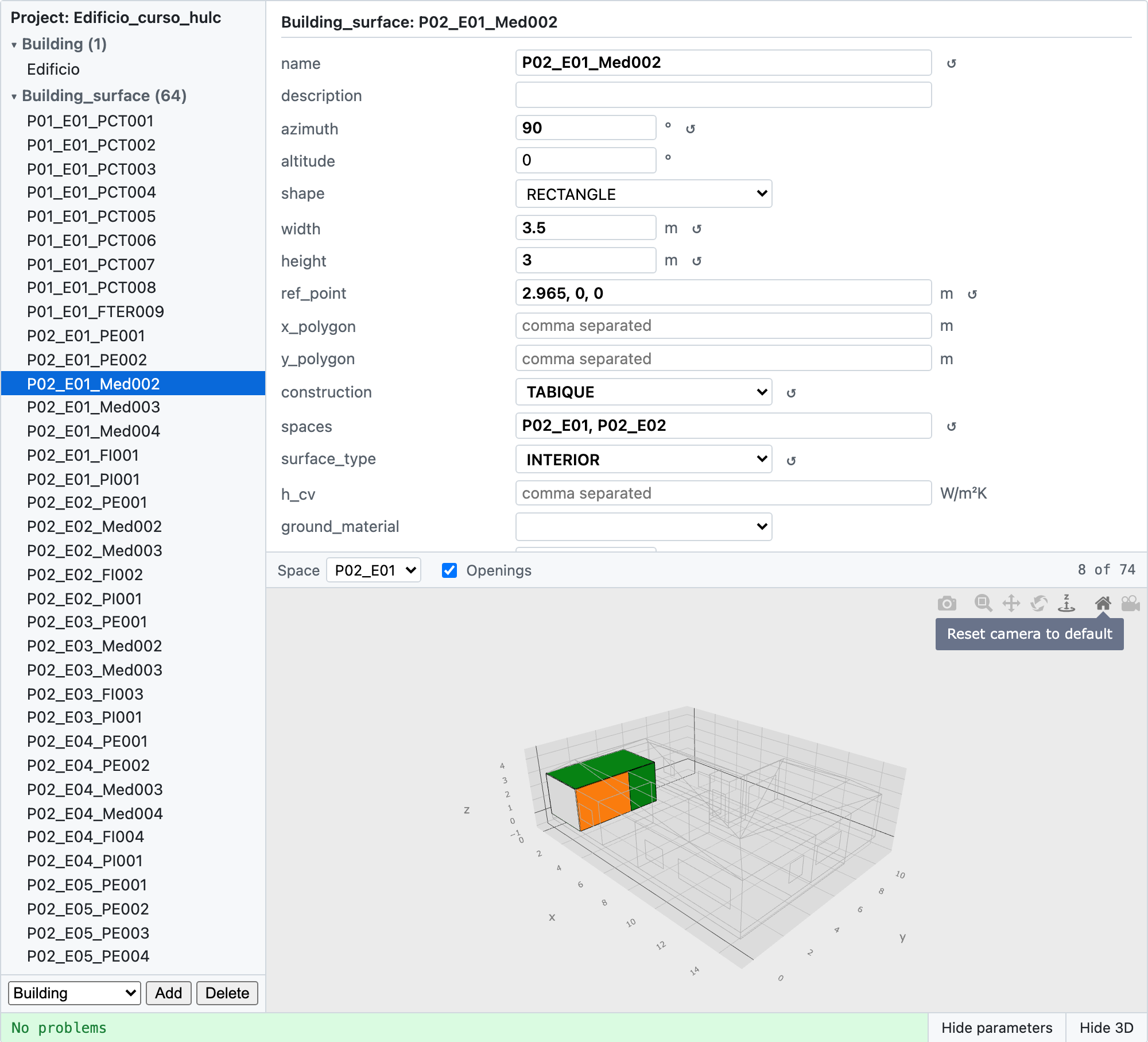
The Space dropdown shows one space at a time, which is the way to see interior partitions: from outside, the exterior walls hide every surface behind them. The rest of the building stays as a grey wireframe, so the space keeps its place and its size in a recognisable model, and only the surfaces of the chosen space answer the mouse. Openings hides the windows and doors.
The selection is linked both ways: picking a component in the list paints it orange in the view, and clicking a surface in the view selects it in the list and shows its parameters.
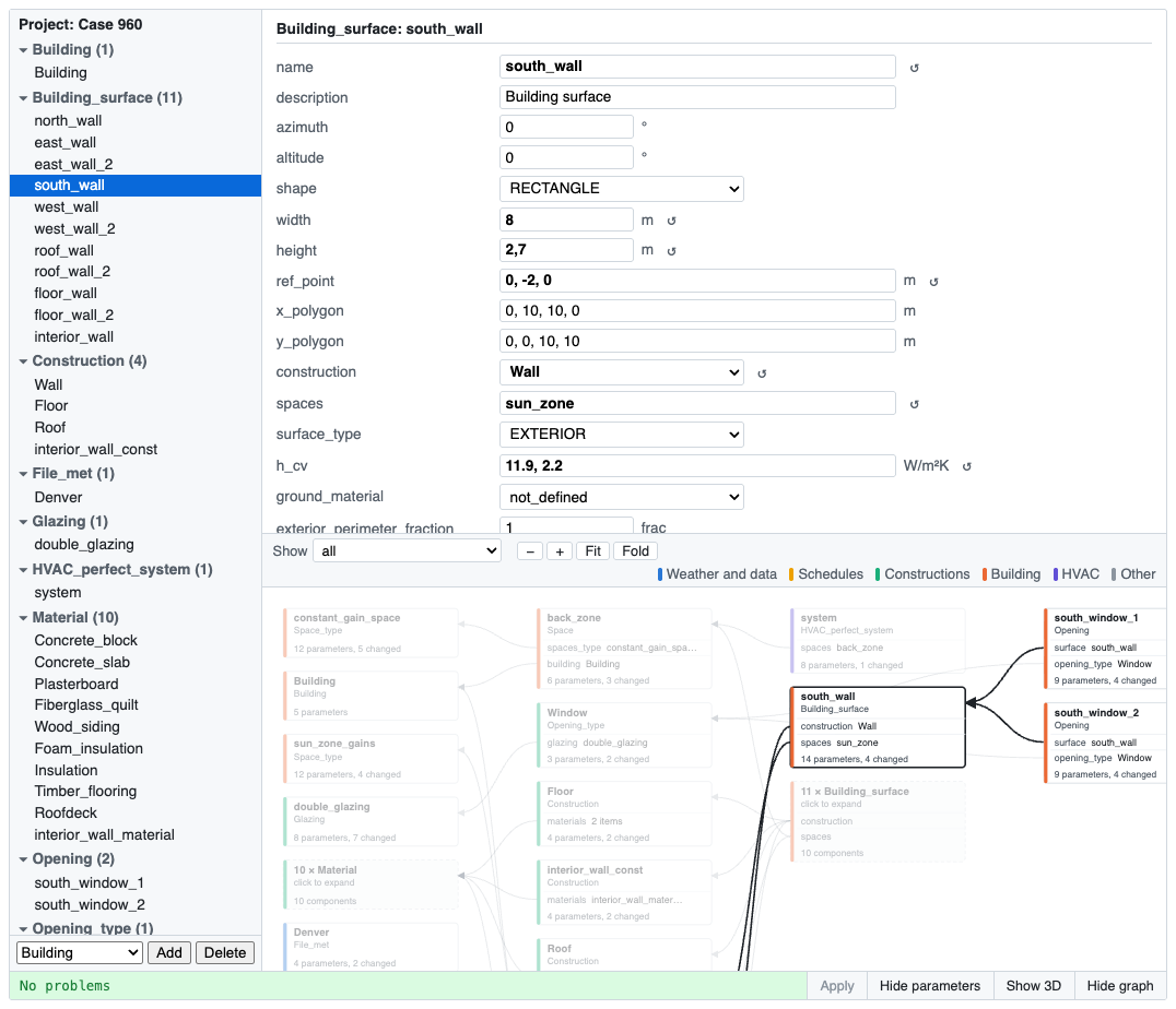
The Show graph button shows, in the same place, a graph of the components: one box per component, with its name and type, a row for every parameter that refers to other components (construction, spaces, materials…) and how many of its parameters differ from the default. An arrow goes from each of those rows to the component it names, and the boxes are laid out in layers, so that what a component uses is always to its left: materials, schedules and weather on the left, then constructions, spaces, surfaces and openings, and the systems on the right. The colour of the left edge of a box tells its family (legend in the bar); clicking a family in the legend hides its components and their arrows, and clicking it again shows them (the selected component is always shown).
The graph shows the document being edited, so it follows every change at once. A type with more than six components is folded into one box ("64 × Building_surface"); clicking it shows them one by one, and Fold folds them again. Clicking a box selects the component in the list and in the form, and lights up its arrows and the components at their ends; selecting a component in the list or in the 3D view does the same in the graph. Clicking the empty background clears the selection. Show: selected and what it uses keeps only the selected component, everything it uses down to the materials, and the components that use it. Drag to move the graph; the − / + buttons, or Ctrl/⌘ + wheel (pinch on a trackpad), zoom it, and Fit brings it all back into the panel.
The view shows the project, not the document being edited: geometry needs a built model, with references resolved and origins placed relative to the building, which the document alone does not give. Moving a vertex is a plain change of value, so it reaches the project and the view straight away; adding or removing a surface waits for apply(). refresh_geometry() reloads the view after changing the project from code.
The edited definition is available as editor.value, and not every edit reaches the project the same way.
Changing a value — a number, a dropdown, a list of coordinates — is a local assignment, so it is put into the project as you edit, with nothing to press. The component stays the same object, so a variable holding it does not go stale and its results are not thrown away.
Renaming, adding or removing a component, or changing its type needs the project rebuilt, because components refer to each other by name and those references are resolved when the definition is loaded. Those wait: the bar turns amber saying what is missing, the Apply button lights up, and editor.pending lists them. The button is also disabled while the document does not satisfy the schema, since applying would be refused anyway.
editor.apply() does the same as the button, and can also be called from the notebook:
editor = pro.editor()
editor                       # edit it in the notebook
...
errors = editor.apply()      # rebuild pro from the edited definition
It validates the document first and leaves the project untouched if it does not satisfy the schema, so a half applied definition cannot happen; in that case it returns the schema errors. Otherwise it returns the messages from check(). The project is rebuilt rather than patched, so any variable holding a component from before has to be asked for again with pro.component(name), and any simulation results are dropped along with the components they came from.
A value that does not satisfy the schema never reaches the project either. It stays in the document, marked under its field, and goes in as soon as it is corrected.
editor.validate() gives the schema errors of the document, and editor.is_valid() whether there are any. Both are computed in Python, so they also work in a script, without a browser having rendered the widget.

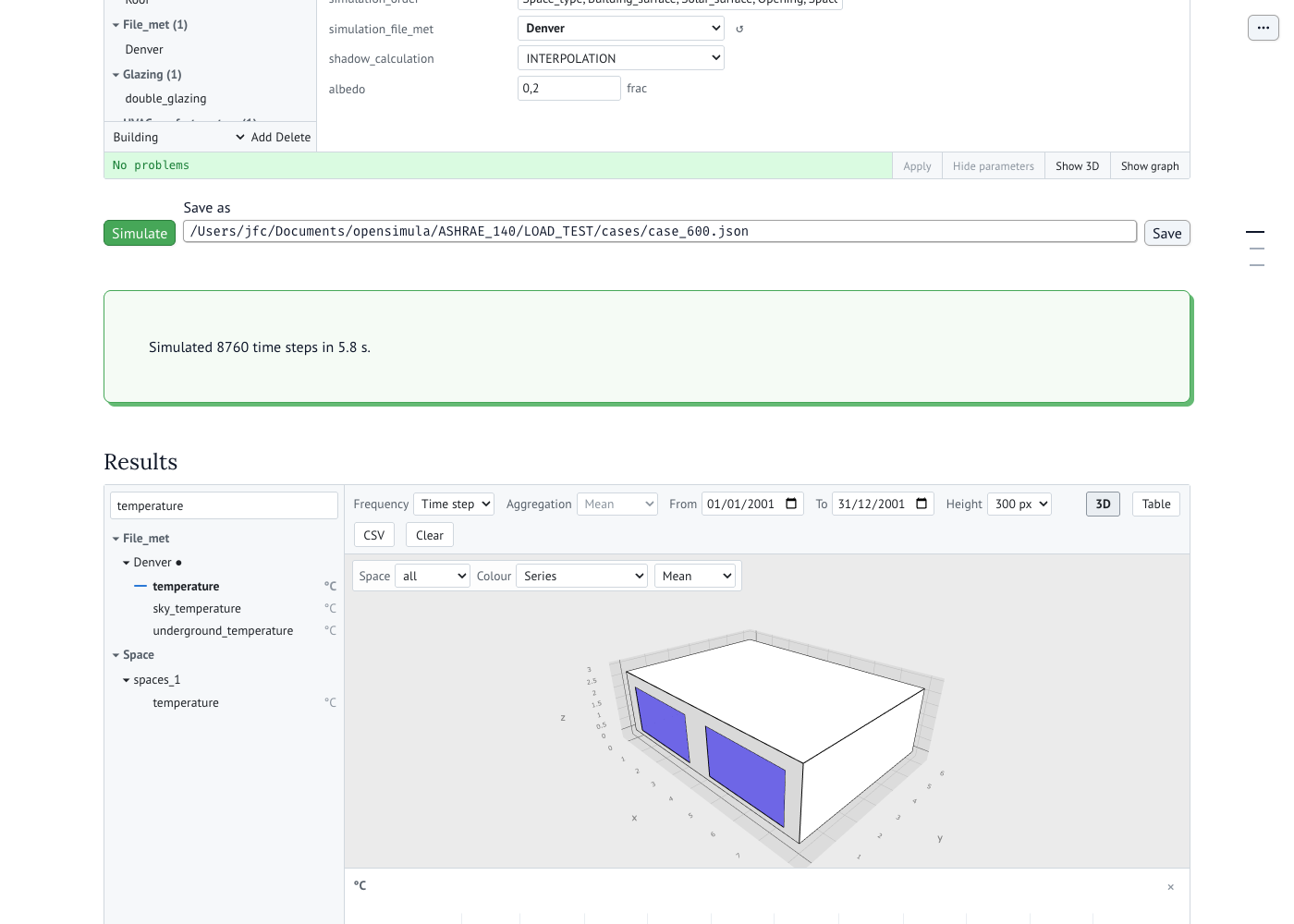
- results(*variables, height=600, chart_height=300): Returns an interactive viewer of the results of a simulated project, displayed directly in Jupyter or wrapped in
mo.ui.anywidget(...)in Marimo. The components with results are listed on the left, grouped by type, with a filter box; clicking a variable adds it to the charts and clicking it again removes it. The variables can also be given as arguments, as"component.variable". Up to 8 variables are shown at the same time, one chart per unit (temperatures together, powers together), and each variable keeps its colour while it stays selected.
pro.simulate()
viewer = pro.results("spaces_1.temperature", "Denver.temperature", "system.Q_sensible")
viewer
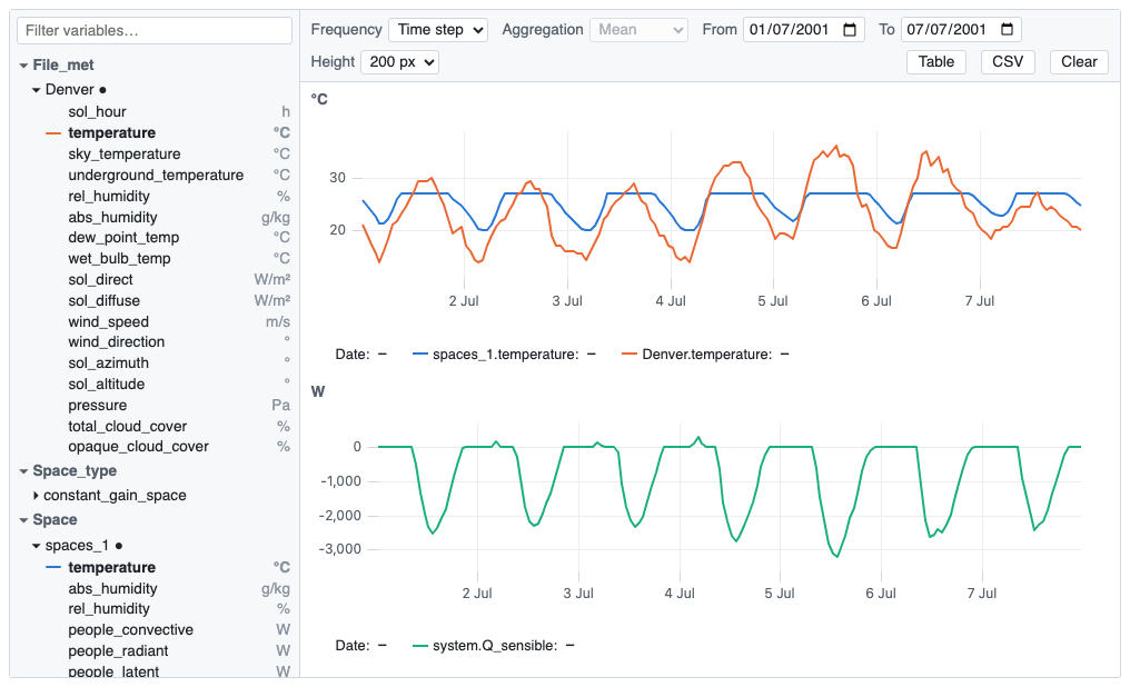
The toolbar sets the Frequency ("Time step", hourly, daily, monthly or yearly) and the Aggregation used to resample (mean, mean without zeros, sum, sum of positives, sum of negatives, max or min; each period is labelled by its start; the sums of positives and of negatives tell apart heating and cooling in a variable with sign, and the mean without zeros leaves out the hours a variable is 0, such as the EER of a unit while it is off), the From/To dates of the interval shown, and the Height of each chart. Monthly and yearly values are drawn as bars, one per period, side by side when a chart has several variables. Table switches to a table of the values shown, and CSV downloads them.
In the charts, the legend gives the values under the cursor; clicking a legend entry hides or shows that variable, and Shift + click removes it. The × at the top right of a chart removes all its variables. Drag horizontally to zoom in on a period, Shift + drag to move it in time, and double-click to go back to the whole interval; zooming or moving one chart applies to all of them.
Everything can also be set from Python, and the viewer updates itself:
viewer.select("spaces_1.rel_humidity")       # add variables
viewer.frequency = "daily"                   # "none", "hourly", "daily", "monthly", "yearly"
viewer.aggregation = "max"                   # "mean", "mean_nonzero", "sum", "sum_pos", "sum_neg", "max", "min"
viewer.interval = ["2001-07-01", "2001-07-31"]  # [] for the whole simulation
viewer.chart_height = 400                    # pixels of each chart
viewer.height = 750                          # pixels of the whole viewer
df = viewer.dataframe()                      # the values shown, as a pandas DataFrame
The 3D button (or pro.results(..., show_3d=True), or viewer.show_3d = True) shows the geometry of the project above the charts. Clicking a surface or a window there opens it, and the spaces it belongs to, in the list on the left, ready to pick its variables. The surfaces whose variables are plotted are drawn in the colour of their series, and the outline of a space whose variables are plotted takes its colour too, so the charts and the model can be read together.
The Colour selector at the top left of the 3D view colours the surfaces by one of their variables instead (viewer.color_variable = "T_s0"), with its mean, maximum or minimum over the interval shown (viewer.color_statistic), or At cursor ("instant"): the model then follows the cursor of the charts, coloured with the values at the time under it (shown next to the selector), on one scale for the whole interval so that two instants can be compared. With this option the series of all the surfaces are sent to the browser, at the frequency of the charts, so for a large building a shorter interval or a coarser frequency keeps it light. The scale has one hue when all the values have the same sign, and two hues around a grey zero when they have both, as heat flows do; windows are drawn opaque, surfaces without that variable are drawn as an outline only, and hovering a surface gives its value. The Space selector shows one space alone, with the rest of the building as an outline, which is the way to see its interior surfaces.
After simulating the project again, viewer.refresh() reloads the variables.
-
geometry_dict(): Returns the geometry of the project as plain data,
{"meshes": [...], "spaces": [...]}, with one mesh per polygon: its triangles, its outline, its colour, and the component and the spaces it belongs to. It is what feeds the 3D view of the editor, and it is available on its own for any other viewer. -
show_3D(): Displays an interactive 3D Plotly visualization of all the components with 3D representation, like Buildings: rendered inline when called from a Jupyter notebook, or opened in a browser tab otherwise.
-
plotly_figure_3D(): Same view as
show_3D(), returned instead of shown, so it can be composed, saved, or otherwise reused. -
show_3D_shadows(date): Calculates and displays an interactive 3D Plotly visualization of the buildings with the shadows occurring for the date specified. date: Python datetime object specifying a specific date.
-
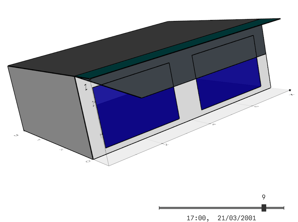
show_3D_shadows_animation(date): Calculates and displays an interactive 3D Plotly visualization of the buildings with the shadows occurring for the day date specified, with the slider bar at the bottom, you can change the time of day and see an animation of the shadows. date: Python datetime object specifying a specific date. See next figure as example:
the first simulation instant is the initial_time plus 1/2 of the time_step. For example, if initial_time = “01/01/2001 00:00:00” and time_step = 3600, then the first simulation instant is: “01/01/2001 00:30:00”, the second: “01/01/2001 01:30:00”, and so on.
OpenSimula app
The editor and the results viewer can also be used without writing a notebook, put together in an app that opens in the browser. It needs marimo, installed with the gui extra:
pip install "opensimula[gui]"
opensimula gui project.json
The Examples are a good place to start: opensimula examples copies them to a folder, ready to open. The project file is optional: without it the app starts with an empty project, and Open or create a project opens another JSON file or starts a new one. The page has, from top to bottom:
- The editor of the project, with its 3D view and its graph, exactly as
pro.editor(). - Simulate, which applies every edit to the project, checks it and simulates it, with a progress bar. Problems found by the check are listed instead of simulating, and the warnings of the simulation (time steps that did not converge…) under the time it took.
- Save, which writes the document being edited to the JSON file given next to it (the file opened, by default), even if it still has problems.
- The results viewer, as
pro.results(). It stays the same across simulations: after changing a parameter and simulating again, the variables already plotted, the frequency, the interval and the 3D view are kept, and show the new values.
Relative file names in the project, such as the weather file of File_met, are read from the folder the command is run from (the working folder, shown at the top), as they are in a notebook. To open an ASHRAE 140 case, for example, run it from its test folder: cd ASHRAE_140/LOAD_TEST and opensimula gui cases/case_600.json. --port chooses the port of the app server and --headless does not open a browser; Ctrl+C in the terminal stops it.
Components
Components are objects included in projects that contain parameters and variables. Component list describe the different types of Components in opensimula.
As an example, we will see how to create three different types of components and how to manage them in our project. this code is a continuation of the definition of the previous project.
...

working_day = pro.new_component("Day_schedule","working_day")
param = {
    "time_steps": [8*3600, 5*3600, 2*3600, 4*3600],
    "values": [0, 100, 0, 80, 0]
}
working_day.set_parameters(param)

holiday_day = pro.new_component("Day_schedule","holiday_day")
param = {
    "time_steps": [],
    "values": [0]
}
holiday_day.set_parameters(param)

week = pro.new_component("Week_schedule","week")
param = {
    "days_schedules": ["working_day","working_day","working_day","working_day","working_day","holiday_day","holiday_day"]
}
week.set_parameters(param)

year = pro.new_component("Year_schedule","year")
param = {
    "periods": [],
    "weeks_schedules": ["week"]
}
year.set_parameters(param)
To create the components we use project "new_component" function. For example, to create a Day_schedule we will use pro.new_component("Day_schedule","name"). Where the first argument is the type of component and the second the name of the component.
After creating the components we can modify any of their parameters.
After defining a project with its components, changing the parameters one by one or using a dictionary to define it, we can check if there is any error using the check() function and perform the temporary simulation with the simulate() function.
...

pro.check()
pro.simulate()
Python shell output:
Checking project: Project 1
Checking completed.
Simulating Project 1: ...
100%|██████████| 52560/52560 [00:26<00:00, 1960.14step/s, n_iter=1]
The list of parameters of a project can be obtained in pandas DataFrame format using the project functions parameter_dataframe(). For the components we can get parameters and variables dataframes with parameter_dataframe() and variable_dataframe().
To obtain the list of components in a project with the parameters as columns use the function component_dataframe(comp_type="all").
In the "type" argument of the function we can indicate the type of components we want to list (for example: "Day_schedule"), or indicate "all" (this is the default value), which will show all components including only the three parameters common to all components: "name", "type" and "description".
With Jupyter notebooks or Google Collab, writing the python variable of a project the parameter and component dataframe will be shown, and writing one component python variable parameter and variable dataframe will be shown. Next example shows the parameter and component dataframes of our project:
...

pro
Jupyter shell:

Components functions
The following is a list of the most useful functions of the Components object:
- parameter(name): Returns the parameter "name".
- parameter_dataframe(): Returns pandas DataFrame with the parameters of the component.
- set_parameters(dict): Change component parameters using python dictonary.
- check(): Returns the list of errors after checking the components. All the errors returned are also printed.
- variable(name): Returns the variable "name".
- variable_dataframe(units=False, frequency=None, value="mean", interval=None, pos_neg_columns=[]): Returns a pandas dataframe with all the variables of the component.
This is the meaning of the arguments of the variable_dataframe function. (In bold the default values):
- units [False/True]: Include de units in the name of the variable.
- frequency [None, "hourly", "daily", "monthly", "yearly"]: Frequency of the data, that of the simulation (None), hourly, daily, monthly or yearly.
- value ["mean","max","min","sum","sum_pos","sum_neg"]: If we use a frequency other than the simulation frequency (e.g. "monthly"), the value obtained for each row (month) will be the mean ("mean"), the maximum ("max"), the minimum ("min"), the sum ("sum"), the sum of positive values ("sum_pos") or the sum of negative values ("sum_neg").
- interval [None,[start_date, end_date]]: List with the start and end dates of the period to be included in the dataframe, if the value is None all values are included.
- pos_neg_columns [[]]: List of variables that will be included in separate columns positive and negative values, with "column_name"_pos and "column_name"_neg as names.
Parameters
Parameters are used to define the characteristics that make up the projects and components.
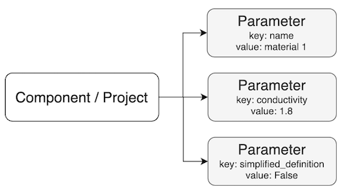
The parameters will be defined as Python dictionary keys (or json format files), that is the format we will use in the examples shown in the documentation. Parameters can be of different types depending on the type of information they contain:
- Parameter_string: String of characters, e.g.:
"name": "Project 1". - Parameter_boolean: True or False value, e.g.:
"simplified_definition": False. - Parameter_int: Integer value, e.g.:
"time_step": 3600. - Parameter_float: Floating point value, e.g.:
"conductivity": 1.8. - Parameter_options: character string included in a closed option list, e.g.:
"file_type": "EXCEL". - Parameter_component: Reference to another component, e.g.:
"meteo_file": "Sevilla". - Parameter_variable: This parameter is used to create a variable in the component by copying it from another component. A new name is defined and the unit will be taken from the original variable. e.g.:
"input_variables": "t_1 = meteo.temperature", a variable called "t_1" will be created which is a copy of the variable "temperature" of the component "meteo". - Parameter_math_exp: parameter defining a mathematical expression. Each of the components knows how to use that mathematical expression within its simulation process. e.g.:
"people_density": "0.1 * f", this parameter states that the people density shall be calculated by multiplying by 0.1 a variable called "f" that the component must include. The mathematical expressions must be written in Python.
All of the above types can also be defined as parameter lists, giving rise to the following types:
- Parameter_string_list: List of String of characters, e.g.:
"authors": ["Juan F.", "Luis", "Ismael"]. - Parameter_boolean_list: List of True or False values, e.g.:
"operated": [True, True, False]. - Parameter_int_list: List of integer values, e.g.:
"people": [24, 12, 18]. - Parameter_float_list: List of floating point values, e.g.:
"solar_alpha": [0.8, 0.75]. - Parameter_options_list: List of character strings included in a closed option list, e.g.:
"day_types": ["MONDAY", "TUESDAY"]. - Parameter_component_list: List of references to another components, e.g.:
"materials": ["Cement mortar", "Hollow brick"]. - Parameter_variable_list: List of parameters used to copy a list of variables. e.g.:
"input_variables": ["t_1 = meteo.temperature","hr = meteo.relative_humidity"]. - Parameter_math_exp_list: List of mathematical expressions. e.g.:
"curves": ["0.3 * t + 20","0.04 * t**2 - 0.2 * t + 3 "].
The Parameter_component, Parameter_variable, Parameter_component_list and Parameter_variable_list can refer to a component of the same project, in that case it is only necessary to put the name of the component, or a component of another project. In this last case we must write "project_name->component_name". e.g. "meteo_file": "Project 1->Sevilla".
To get or set the value of a parameter we must use the attribute "value" of the parameter. If the parameter contain a list we can set/get each value using index, for example: pro.component("week").parameter("days_schedules").value[0] will return "working_day"
...

pro.component("year").parameter("description").value = "Example of year schedule"
pro.component("year").parameter("description").value
Jupyter output:
'Example of year schedule'
Variables
Variables are elements included in the components to store the temporal information generated during the simulation.
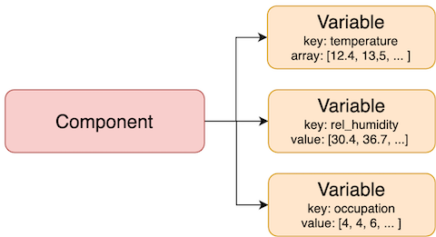
Variables are lists of floating values, one for each instant of simulated time.
To access the values of a variable we use the values attribute which returns a numpy.array object (NumPy library array object).
...

pro.component("year").variable("values").values
Jupyter output:
array([  0.,   0.,   0.,   0.,   0.,   0.,   0.,   0.,   0.,   0.,   0.,
         0.,   0.,   0.,   0.,   0.,   0.,   0.,   0.,   0.,   0.,   0.,
         0.,   0.,   0.,   0.,   0.,   0.,   0.,   0.,   0.,   0., 100.,
       100., 100., 100., 100., 100., 100., 100., 100., 100., 100., 100.,
       100., 100., 100., 100., 100., 100., 100., 100.,   0.,   0.,   0.,
         0.,   0.,   0.,   0.,   0.,  80.,  80.,  80.,  80.,  80.,  80.,
        80.,  80.,  80.,  80.,  80.,  80.,  80.,  80.,  80.,  80.,   0.,
         0.,   0.,   0.,   0.,   0.,   0.,   0.,   0.,   0.,   0.,   0.,
         0.,   0.,   0.,   0.,   0.,   0.,   0.,   0.,   0.,   0.,   0.,
         0.,   0.,   0.,   0.,   0.,   0.,   0.,   0.,   0.,   0.,   0.,
         0.,   0.,   0.,   0.,   0.,   0.,   0.,   0.,   0.,   0.,   0.,
         0.,   0.,   0.,   0.,   0.,   0.,   0.,   0.,   0.,   0.,   0.,
         0.,   0.,   0.,   0.,   0.,   0.,   0.,   0.,   0.,   0.,   0.,
         0.,   0.,   0.,   0.,   0.,   0.,   0.,   0.,   0.,   0.,   0.,
         0.,   0.,   0.,   0.,   0.,   0.,   0.,   0.,   0.,   0.,   0.,
         0.,   0.,   0.,   0.,   0.,   0.,   0.,   0.,   0.,   0.,   0.,
         0.,   0.,   0.,   0.,   0.,   0.,   0.,   0.,   0.,   0.,   0.,
         0.,   0.,   0.,   0.,   0.,   0.,   0.,   0.,   0.,   0.,   0.,
         0.,   0.,   0.,   0.,   0.,   0.,   0.,   0.,   0.,   0.,   0.,
         0.,   0.,   0.,   0.,   0.,   0.,   0.,   0.,   0.,   0.,   0.,
         0.,   0.,   0.,   0.,   0.,   0.,   0.,   0.,   0.,   0.,   0.,
         0.,   0.,   0.,   0.,   0.,   0.,   0.,   0.,   0.,   0.,   0.,
         0.,   0.,   0.,   0.,   0.,   0.,   0.,   0.,   0.,   0.,   0.,
         0.,   0.,   0.,   0.,   0.,   0.,   0.,   0.,   0.,   0.,   0.,
         0.,   0.,   0.,   0.,   0.,   0.,   0.,   0.,   0.,   0.,   0.,
...
       100.,   0.,   0.,   0.,   0.,   0.,   0.,   0.,   0.,  80.,  80.,
        80.,  80.,  80.,  80.,  80.,  80.,  80.,  80.,  80.,  80.,  80.,
        80.,  80.,  80.,   0.,   0.,   0.,   0.,   0.,   0.,   0.,   0.,
         0.,   0.,   0.,   0.,   0.,   0.,   0.,   0.,   0.,   0.,   0.,
         0.])
Output is truncated. View as a scrollable element or open in a text editor. Adjust cell output settings...
The variable_dataframe(units, frequency, value, interval, pos_neg_columns) method of the components returns a pandas dataframe with all the variables of the component.
As an example we can see how to obtain the monthly average values of the variables of a meteorological file (File_met component):
...

pro.component("met_file").variable_dataframe(frequency="monthly",value="mean")
Jupyter shell:

HVAC systems and water plants
The HVAC components are of two kinds: equipment components, which only hold the manufacturer's data of a piece of equipment and are not simulated by themselves (DX_unit, Water_coil, Fan, Pump, Chiller_heat_pump, Boiler), and systems (HVAC_*), which use them, are simulated in each time step and store the variables of the installation. An installation is put together by references between them:
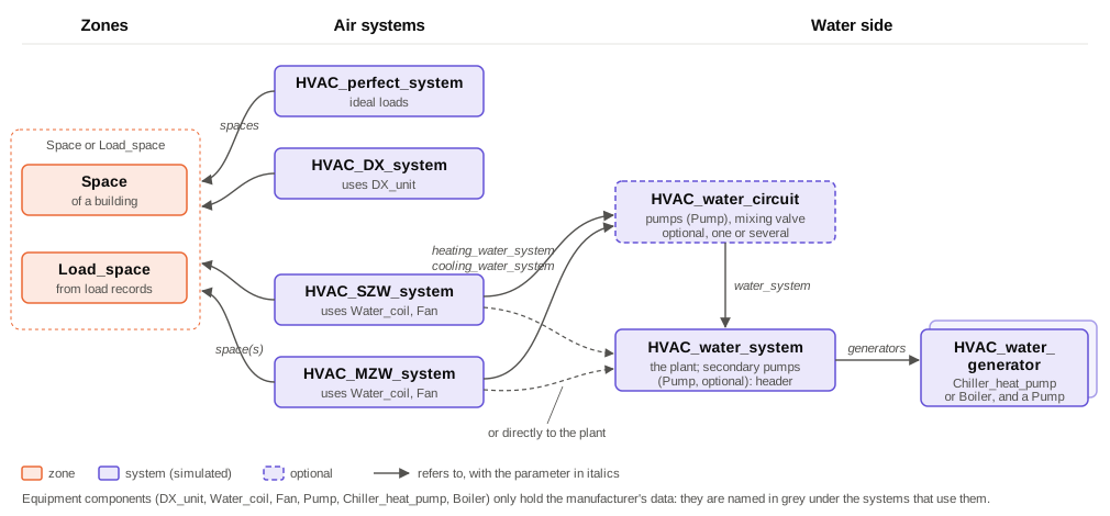
Zones. An air system serves a Space of a building or a Load_space, a zone defined by load records (sensible and latent loads read, for example, from a File_data), which allows to simulate an installation without the building. Both offer the systems the same: their temperature and humidity, and their balance equations. See example 08.
Air systems. HVAC_perfect_system gives exactly the load (ideal loads, example 05); HVAC_DX_system is an air-to-air heat pump (example 06); HVAC_SZW_system (one zone) and HVAC_MZW_system (several zones, with VAV and reheat) have water coils. With water_source "WATER_SYSTEM" (and reheat_water_source for the reheat coils) their coils take the inlet water temperature from a water plant or circuit and give it their load in each iteration; with "UNKNOWN" they use fixed water temperatures.
Water plant. An HVAC_water_system heats and/or cools water with its generators:
- Each
HVAC_water_generatorhas an equipment component, aChiller_heat_pump(electric, heating and/or cooling according to itschiller_type) or aBoiler(fuel, heating only, efficiency on the lower heating value that may depend on the return temperature for condensing boilers), its own pump and its availability, and may have several identical units (number_of_units). - The generators able to serve the mode share the load with the
sequencingof the plant: "PRIORITY", in the order of the list, the next one when the previous is at full load (a heat pump first and a boiler as backup), or "EQUAL_LOAD", all of them at the same part load. When they cannot reach the setpoint they give their full capacity at the actual water temperature. - The mode, heating or cooling, follows the load of the coils ("LOAD_CONTROL") or a schedule ("SCHEDULE_CONTROL", e.g. heating and cooling seasons of a two-pipe installation). Heating and cooling at the same time need two plants (four pipes). Coils only take heat or cold from a plant that can give it in its mode.
- Without secondary
pumpsthe water of the coils goes through the generators, moved by their pumps. With them the plant has a header between the primary circuit of the generators and the secondary one: the primary pump of each generator moves water only while it runs, and the mixing in the header matters. A primary flow larger than the secondary returns hot water to the generators through the bypass (bad for a condensing boiler); a smaller one sends part of the return to the supply (the water to the coils is below the setpoint).
Circuits. An HVAC_water_circuit hangs from a plant: its own pumps, availability and, with a mixing valve (heating_supply_setpoint, cooling_supply_setpoint), its own supply temperature. A plant can feed several circuits at different temperatures. For the coils a circuit is like a plant; for the plant it is one more coil.
Results. Each component stores its own variables: each generator its load, part load, electric and fuel power and efficiency; each circuit its temperatures, flows and the load it gives to the plant; the plant the temperatures of the supply, return and generators, the flows of the primary, secondary and bypass, the balance of its water and the total electric (electric_power) and fuel (generators_fuel_power) power. The water balance of a plant is delta_U = Q_generators + Q_coils + Q_process + Q_loss + Q_pump.
As an example, the water side of example 09: a heat pump first, a condensing boiler as backup, and a circuit at 45 °C at most.
...

pro.new_component("HVAC_water_generator", "heat_pump_generator").set_parameters(
    {"equipment": "heat_pump", "pump": "heat_pump_pump"})
pro.new_component("HVAC_water_generator", "boiler_generator").set_parameters(
    {"equipment": "boiler", "pump": "boiler_pump"})
pro.new_component("HVAC_water_system", "water_plant").set_parameters({
    "generators": ["heat_pump_generator", "boiler_generator"],
    "sequencing": "PRIORITY",
    "heating_water_setpoint": "50",
    "cooling_water_setpoint": "7",
    "total_water_volume": 50,
    "system_control": "LOAD_CONTROL",
})
pro.new_component("HVAC_water_circuit", "south_circuit").set_parameters({
    "water_system": "water_plant",
    "pumps": ["south_pump"],
    "heating_supply_setpoint": "45",
})
# the fan coil (HVAC_SZW_system) refers to the circuit
pro.component("fan_coil_south").set_parameters({
    "water_source": "WATER_SYSTEM",
    "heating_water_system": "south_circuit",
    "cooling_water_system": "south_circuit",
})
The parameters and variables of every component are in the component list.